Here’s a quick guide on how to merge cells in Google Sheets in different ways.

In a nutshell:

Select the cells you want to merge.
Click the “Merge cells” button.
Choose the merge type: all, horizontally, or vertically.

How to Merge Cells in Google Sheets on Desktop

It couldn’t be easier:

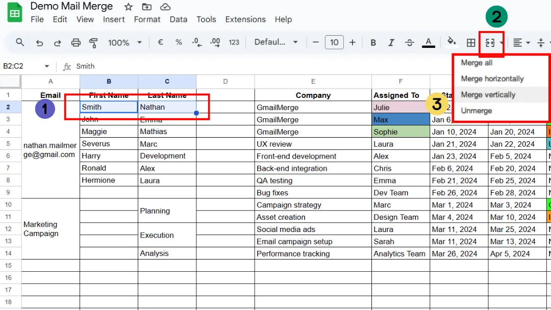
Select the cells you want to merge.
Click the “Merge cells” button.
Choose the merge type:

Merge all → all selected cells become a single cell.
Merge horizontally → merges across the row only.
Merge vertically → merges down the column only.

🚨 Heads up: If you merge cells that already contain data, only the content in the top-left cell will be kept. Everything else will be deleted (which matters if you later mail merge with attachments). This technique is especially useful if you’re preparing data for a mail merge in Gmail, where keeping all the personalized text intact is crucial.

👉 Tip: If you want to keep all the text, you’ll need to combine it with a formula first, and then merge the cells. We’ll cover that in the next section.

How to Merge Cells in Google Sheets without Losing Data

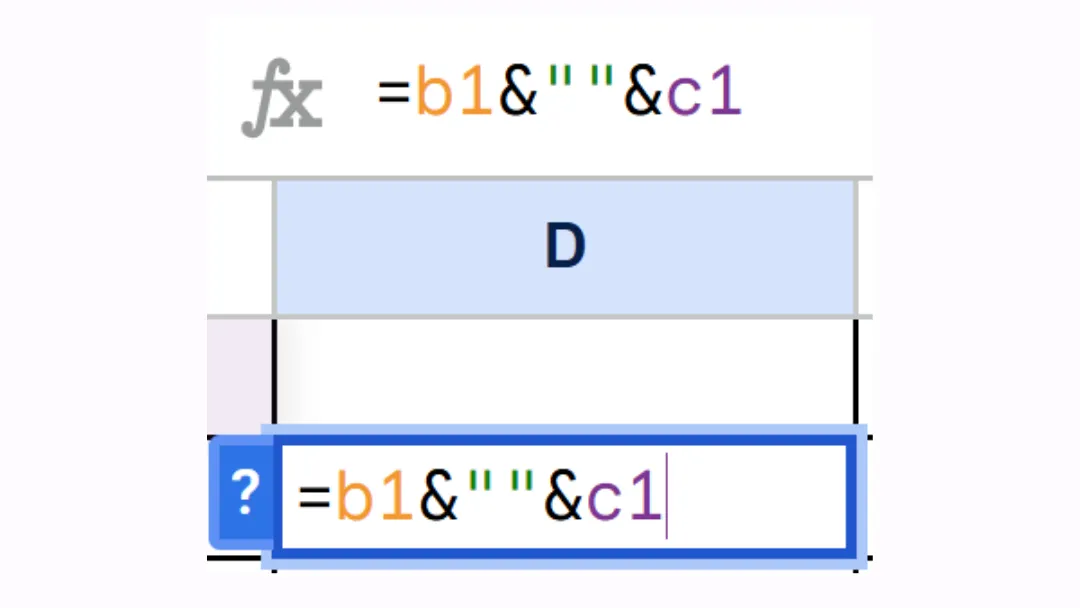
Create a new empty cell, or choose an existing empty cell.
In this new cell, if you want to merge the contents of cells B1 and C1, type the formula:

=B1 & " " & C1

You’ll see the combined text appear.
You can then copy and paste this value (right-click → Paste special → Paste values only) into a cell, and then merge.

How to Merge Cells in the Google Sheets Mobile App

Follow these steps:

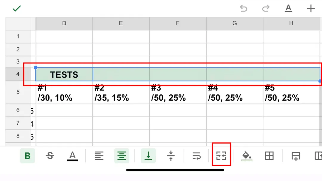
Select the cells you want to merge: tap the first cell, then drag the blue handle to select more.
Tap the format menu icon (toolbar at the top). It looks like a little underlined “A.”
Choose “Merge cells.” A Merge option will appear in the menu.
Tap it to merge your cells.

⚠️ On mobile, you only get one Merge button (there’s no option to choose horizontal vs. vertical like on desktop).

⚡ You can type formulas (like =ARRAYFORMULA(...)) into a cell if you know them, but you can’t easily insert them from a menu. That’s why it’s usually easier to do this on desktop.

How Do I Merge Two Cells into One in Google Sheets

As explained earlier in this article:

Open your Google Sheets file.
Select the two cells you want to merge.
Click the “Merge cells” button.

Why can't I Merge Cells in Google Sheets

There are several reasons why you might not be able to merge cells in Google Sheets. Here are the most common cases:

1️⃣ You’re trying to merge within a protected range.

If the sheet or certain cells are protected by rules (e.g., locked sheet or restricted permissions), the Merge option may be grayed out.
👉 Check if you have editing rights.

2️⃣ The cells are part of a pivot table.

You can’t merge cells inside a pivot table.
👉 First, copy the pivot table into a new sheet as plain values.

3️⃣ The cells are in a filtered range.

When a filter is applied, some actions like merging aren’t allowed.
👉 Temporarily remove the filter.

4️⃣ The cells belong to imported data (linked range).

Example: a range brought in via =IMPORTRANGE() or another external connection.
👉 Copy the data into regular cells first.

5️⃣ Google Sheets blocks it to prevent conflicts.

Example: if you’re trying to merge a very complex block (lots of rows/columns with different data).
👉 Double-check that your selection is correct (e.g., B1:C3 instead of an irregular range).

How to Merge Cells and Keep All Text

This is a common pitfall in Google Sheets: only the content of the top-left cell is preserved, and everything else disappears.

The solution is to combine the text with a formula before merging.

Case 1: Merge Two Cells and Keep Both Texts

Example:

Cell A1: Last Name

Cell B1: First Name

Step 1: Choose or create a new empty cell (e.g., C1).
Step 2: Type the formula:

=A1 & " " & B1

→ This will display the content of A1 followed by a space and the content of B1, i.e.: Last Name First Name.

💡 You can change the separator:

", " → adds a comma and space → Last Name, First Name.
" - " → adds a dash → Last Name - First Name.

Case 2: Merge multiple rows and keep all texts

Example: You want to merge and keep the text from columns B and C for rows 1 through 10.

Step 1: Choose or create a new empty column (e.g., column D).
Step 2: In the first cell of column D, type the formula:

=ARRAYFORMULA(B1:B10 & " " & C1:C10)

-> This will combine each row side by side (B1 C1, B2 C2, …) into column D.

How to Combine Two Columns in Google Sheets with a Space

Refer back to the previous section “How to Merge Cells and Keep All Text” and you’ll have the answer!

Remember these formulas:

=A1 & " " & B1
=ARRAYFORMULA(B1:B10 & " " & C1:C10)

You can simply change the separator:

", " → adds a comma and space → Last Name, First Name
" - " → adds a dash → Last Name - First Name

How to Combine Two Cells in Google Sheets for First and Last Name

Again, refer back to “How to Merge Cells and Keep All Text.” The same formula applies here!

How to Merge Cells in a Spreadsheet? How to Merge Cells in Excel?

The basics are the same across all tools (Google Sheets, Excel, LibreOffice, etc.):

Select the cells you want to merge.
Click the Merge cells button (often shown as an icon in the toolbar).
Choose the type of merge (all / horizontal / vertical, depending on the software).

That said, there are some differences depending on the tool.

Google Sheets

No direct keyboard shortcut.
Available options: Merge all, Merge horizontally, Merge vertically.
On mobile → only a single Merge button (no detailed choices).

Excel

Merge & Center button under Home > Alignment.
Several variations: Merge & Center, Merge Across, Unmerge Cells.
Keyboard shortcut: Alt + H + M + C.

LibreOffice Calc

Similar button in the toolbar.
Options close to Excel (Merge & Center, Merge only, etc.).

How to Merge Cells in Google Sheets Shortcut

Google Sheets doesn’t have a direct keyboard shortcut (like Ctrl + …) to merge cells.

Merging has to be done from the toolbar with the Merge cells button.

💡 Pro tip to go faster with the keyboard:

Use Alt + / (Windows) or Option + / (Mac) → this opens the menu search bar.
Type Merge → you’ll quickly access the Merge cells option without using your mouse.

Here’s a list of useful keyboard shortcuts in Google Sheets (desktop) related to working with cells:

⌨️ Shortcuts for selecting and navigating:

Ctrl + Space → select entire column.
Shift + Space → select entire row.
Ctrl + A → select entire sheet (press twice if needed).
Shift + Arrow keys → extend selection one cell at a time.
Ctrl + Shift + Arrow keys → extend selection to the end of the data.

✏️ Shortcuts for editing cells:

Ctrl + Enter → enter the same value in all selected cells.
F2 → edit the active cell without double-clicking.
Ctrl + D → copy the value from the cell above into the selection.
Ctrl + R → copy the value from the cell to the left into the selection.

➕➖ Shortcuts for inserting/deleting:

Ctrl + Shift + “+” → insert a new row or column.
Ctrl + “-” → delete the selected row or column.

🔍 Quick search for options (pro tip):

Alt + / (Windows) or Option + / (Mac) → open the menu search bar.

👉 You can type Merge to quickly apply cell merging.

How to Unmerge Cells in Google Sheets

On desktop

Select the merged cell (the one spanning multiple rows/columns).
Click the Merge cells button in the top toolbar.
In the dropdown menu, choose Unmerge.

⚠️ Important: Only the content from the top-left cell will be kept. All other cells will become empty again.

On the mobile app (Android/iOS):

Select the merged cell.
Tap the underlined “A” icon (format menu).
Tap Merge → it works as a toggle:

If the cells are merged → tapping will unmerge them.
If the cells are unmerged → tapping will merge them.

Google Sheets: Merge Two Columns

Merging two columns in Google Sheets saves you from manually copying formulas row by row.

Create a new column, for example column D.
In the first cell of this column (D1), if you want to combine columns B and C, type:

=ARRAYFORMULA(B1:B8 & " " & C1:C8)

-> The entire column D will automatically display the combined content row by row.

Expert Insight: Personalize Your Mail Merge with Gmail and Google Sheets

If you combine the First Name and Last Name columns in Google Sheets, it’s not just about formatting your data—it’s also the first step toward a mail merge.

With a tool like Mail Merge for Gmail, each row in your spreadsheet represents an email.

Group (2).png

You can create a First Name column and a Last Name column, then insert them directly into your email template using merge tags (e.g., {{First Name}} {{Last Name}}).

Group 3 (3).png

👉 The result: your contacts receive a personalized message, like “Hi Marie Dupont”, without any copy-pasting or manual edits.

Now that you know everything about merging cells in Google Sheets, why not take the next step? If you want to go further and turn your data into personalized email campaigns, try Mail Merge for Gmail.

It’s free, with no commitment—and you’ll see just how easy it is to create customized emails straight from your Google Sheet !

How to Merge Cells in Google Sheets (2025)