Alphabetizing in Google Sheets means reorganizing a table without breaking the alignment between rows. The method you choose depends on whether you want to

modify the original table,
create an automatically sorted version,
or simply change the way your data is displayed.

In this guide, I walk you through the 3 methods you can use!

⭐ Key Takeaways:

Manual sorting (A→Z / Z→A) is the most reliable method to reorganize a sheet without mixing up data.
The SORT() formula creates a dynamic, automatically updated sorted version—perfect if your data changes often.
Filters give you a temporarily sorted view, but never change the actual order of the sheet.
Most sorting issues come from mixed data types, blank rows, active filters, or protected ranges.

What Does Alphabetizing Mean in Google Sheets?

Alphabetizing in Google Sheets means reorganizing a list of words or names so they appear in A → Z order (from the first letter to the last) or Z → A (the reverse).

When You Should Alphabetize Data

You’ll use alphabetical sorting when you want to:

organize a list in a logical order,
display information from A to Z,
check whether an item is missing,
quickly locate a specific entry,
prepare a file you want to share or present.

Alphabetizing vs Sorting

In Google Sheets, sorting means the order of the rows actually changes in the sheet. This is not just a visual effect—the data is physically rearranged.

A “visual reorganization” happens when you:

apply a filter,
hide certain rows,
change how your data is displayed,
use a view-based sort that affects only your screen, not the underlying sheet.

👉 This is not a real sort: the original table stays in the same order, but Google Sheets shows you a temporary rearrangement.

💡If you're organizing your data for reporting, you might also want to learn how to make a graph in Google Sheets to visualize your results.

Method 1: Alphabetize Your Table by a Column (Manual Sort A→Z / Z→A)

This is the method that 90% of people should use first.

Step 1: Check Your Table

In this example, we’re going to sort a list of customers alphabetically by email.

For sorting to work properly, your sheet must have a header row. This row identifies the name of each column (Email, First Name, Company, etc.).

Step 2: Select the Entire Table (Very Important)

To avoid mixing up your data:

Click the first cell in your table that contains data.
Hold your mouse and drag to the very last cell of your dataset.
The entire table should now be highlighted.

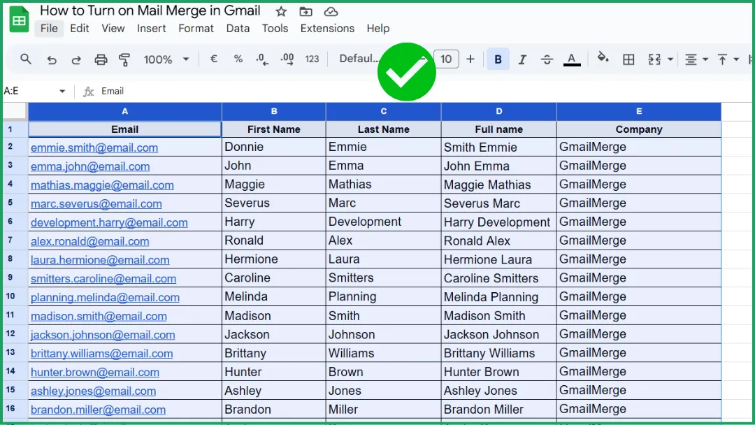
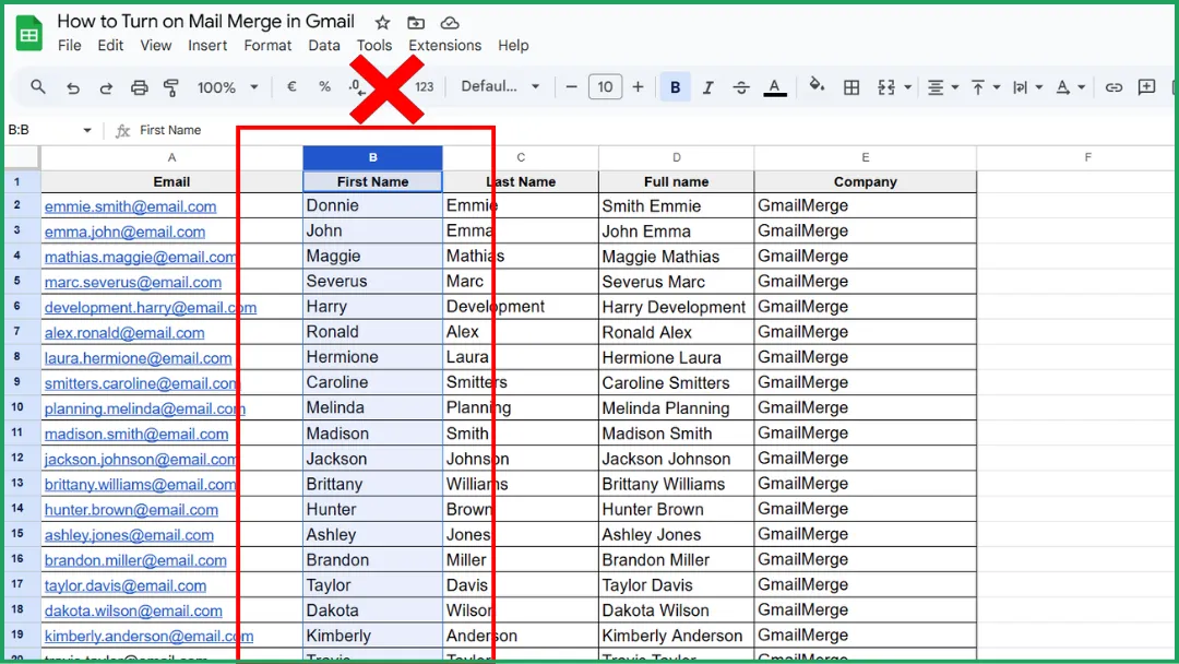
⚠️ Do NOT select only one column. If you sort only one column, Google Sheets will reorder that column but leave the others untouched. Result: the rows no longer match, and your data becomes corrupted.

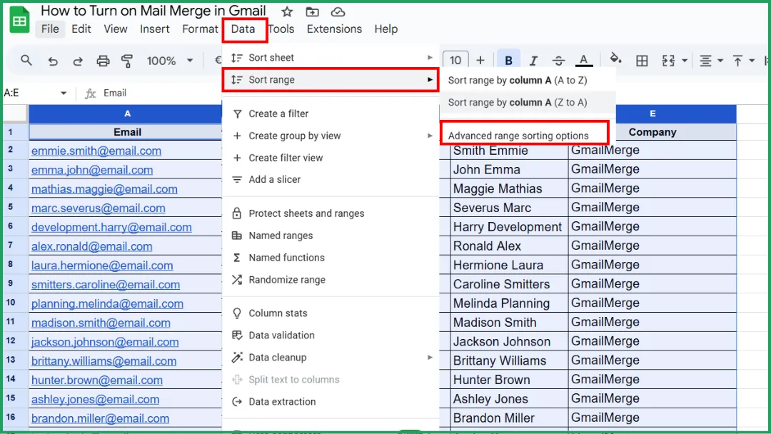
Step 3: Open the Sorting Menu

At the top of Google Sheets:

Click Data.
Click Sort range.
Click Advanced range sorting options.

Step 4: Choose Your Sorting Options

A popup window appears.

Check Data has header row (this keeps your headers in place).
In Sort by, choose the column you want to alphabetize.
Choose the order:

A → Z: alphabetical order from A to Z.

Z → A: reverse alphabetical order.

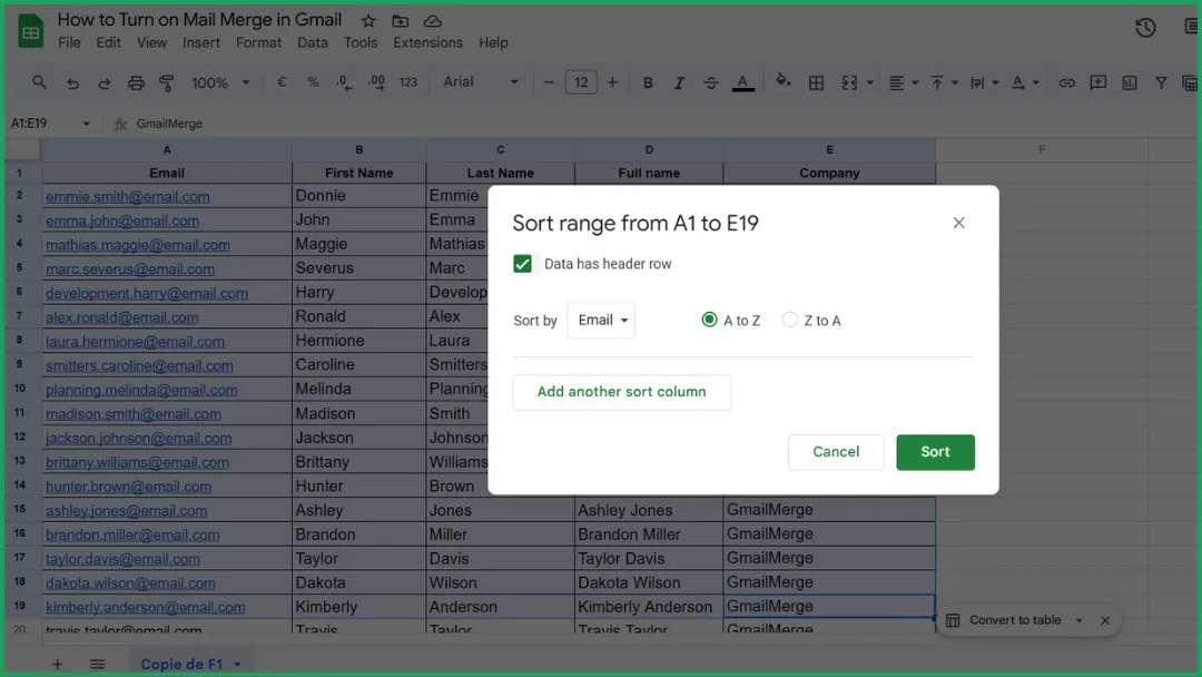
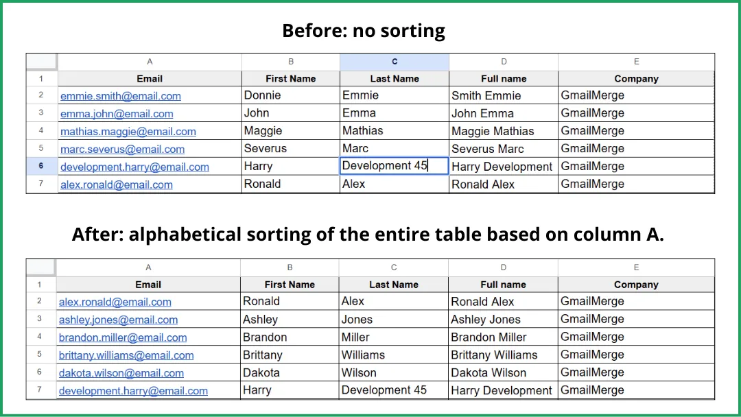
Step 5: Apply the Sort

Click Sort.

Google Sheets will reorganize the entire table based on the column you selected.

Your rows stay perfectly intact, only the order changes.

Alphabetize Your Table Using the Google Sheets Mobile App

The Google Sheets mobile app allows you to sort a range A→Z or Z→A, but with fewer options.

On Android / iOS, you can:

select a range.
open the contextual menu (⋮).
choose Sort range.
choose A → Z or Z → A.

❌ The interface is less intuitive.

❌ Fewer options available (for example: no Data has header row).

Method 2 — Automatically Sort Your Data with the SORT() Formula

With SORT(), you don’t sort your existing table directly.

Instead, you create a new sorted version of your table somewhere else on the sheet (or in a different tab).

The SORT() formula lets you generate a sorted copy without modifying the original data.

When to Use SORT()

✔ When your table updates frequently

✔ When you want to keep the original order untouched

❌ Not ideal if you want to permanently modify the order of the original table (use Method 1 instead)

❌ Not great for sorting a small section of a table, because SORT() forces you to copy the entire range elsewhere — too heavy for small one-off tasks

📌 Real Example: Cold Email Prospecting

Let’s say you manage a Google Sheets prospecting database that fills automatically.

New rows keep arriving at the bottom, unsorted.

But for your cold email campaign, you need a clean list sorted alphabetically (for organization, personalisation, segmentation…).

👉 This is exactly where SORT() is perfect:

your base keeps updating automatically, and your sorted version updates with it.

💡 Why not read our article on cold emails with ChatGPT?

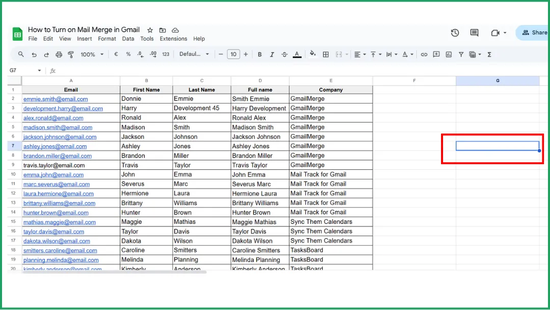
Step 1: Choose Where the Sorted Version Will Appear

Decide where you want your sorted prospect list to show up:

in an empty area to the right of your current table, or
in a brand-new tab.

Click the starting cell — this is where your sorted table will begin (with the same columns as the original).

In this example, we’ll choose an empty cell in the same sheet: G7.

Step 2: Identify the Data Range to Sort

Example:

Your prospect base has:

headers in row 1.
data starting at row 2.
columns from A to E.

👉 Your data range is therefore: A2:E

This automatically includes all existing rows, and the future ones you’ll add.

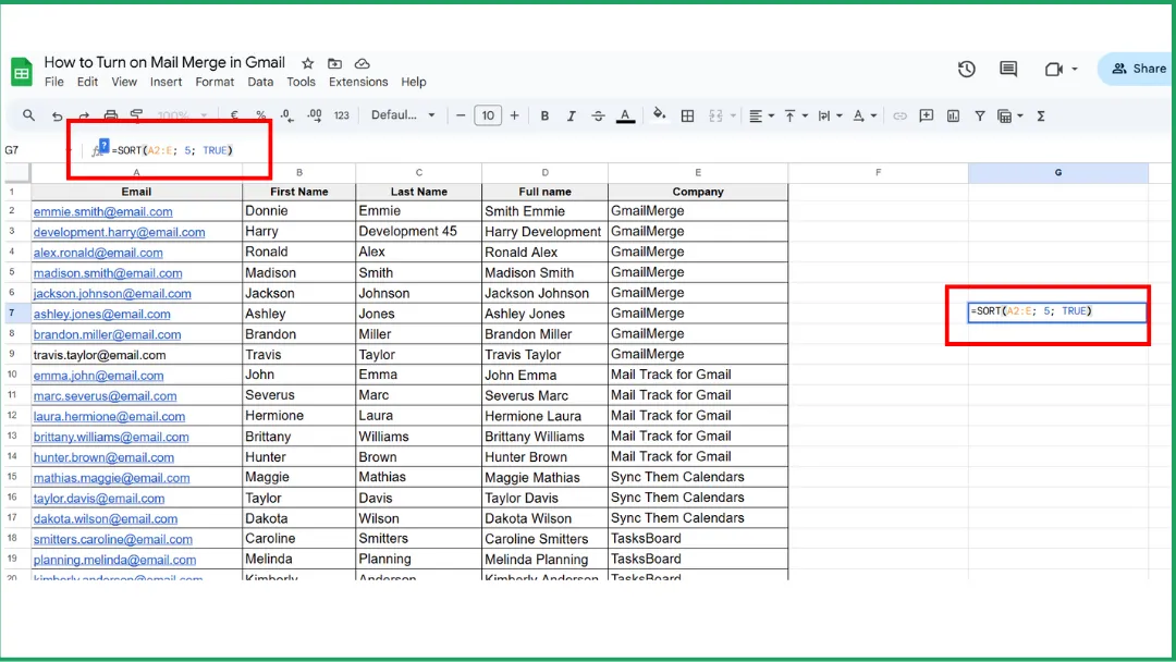
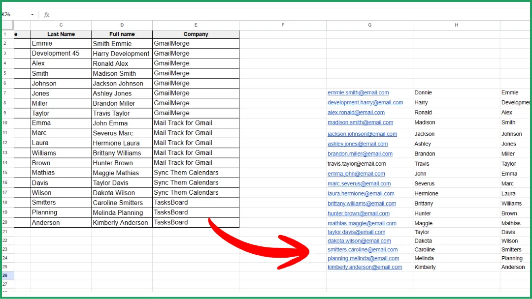
Step 3: Write the SORT() Formula

In this example, we want to alphabetize by Company (column E), from A to Z.

Column “Company” = column E = 5th column in the range.

In an empty cell, type:

=SORT(A2:E; 5; TRUE)

For Z → A sorting, use:

=SORT(A2:E; 5; FALSE)

💡 If your table is large (which is clearly the case here), it’s better to use a new tab.

The formula then becomes:

=SORT('Sheet1'!A2:E, 5, TRUE)

If your tab is named base prospects, the formula becomes:

=SORT('base prospects'!A2:E, 5, TRUE)

You see the pattern? 😉

Step 4: Confirm

Press Enter.

Your sorted version appears instantly.

It updates automatically every time your original table receives new rows.

💡 Once your data is sorted automatically, you can use it directly in Gmail by learning how to mail merge from Google Sheets.

Using SORT() in the Google Sheets Mobile App

✔ 100% supported.

❌ Much less comfortable to type or edit formulas on a phone.

Method 3: Alphabetize Using Filters

This method:

does not modify your table,
does not move any rows,
does not create a new sorted version.

👉 This is NOT a real sort. It simply gives you a temporary view of your data in a different order.

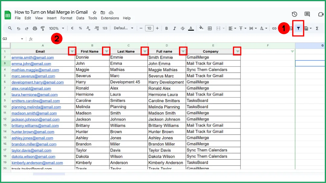
Step 1: Turn On Filters

Click the funnel icon (Filter) in the toolbar.

A dropdown arrow appears in every header cell.

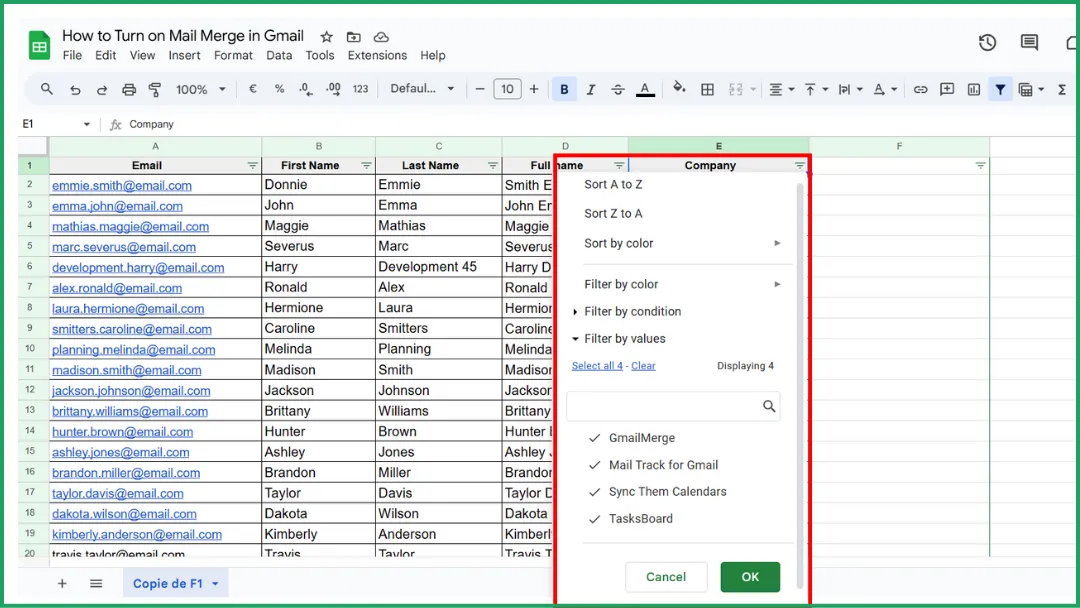
Step 2: Sort Using the Column Arrow

Click the ▼ arrow of the column you want to sort by. Then choose:

Sort A → Z.
Sort Z → A.

This temporarily alphabetizes your view.

Step 3: Turn Off Filters

To disable the filter, simply click the Filter (funnel) icon again.

Your sheet instantly returns to its exact original order.

💡 Good to know: Unlike Method 2 (SORT formula), this method never updates automatically. If you add new rows, you must reapply the filter manually.

Alphabetize Using Filters in the Google Sheets Mobile App

✔ You can apply A→Z / Z→A sorting using filters.

✔ You can turn filters on and off.

So yes, filtering works on mobile…

➡️ but without all the advanced options available on desktop.

💡 If you're wondering how this can help with email personalization, start by understanding what is mail merge is in Gmail here.

Troubleshooting: Alphabetizing Not Working? (Quick Fixes)

Mixed Data Types (Numbers + Text)

Google Sheets sorts differently depending on the type of content. If a single column contains:

Numbers.
Text.
Dates.
cells with invisible spaces.

👉 The sort can behave inconsistently or fail entirely.

💡 Keeping your data clean is also useful if you later need to insert a table in a Gmail message for reporting or summaries.

Hidden Rows or Filters Applied

Sorting may fail or appear incorrect when a filter is still active.

Fix: Turn off all filters.

Protected Ranges

Some cells may be protected (by you or a collaborator). In that case, Google Sheets prevents sorting to avoid breaking important data.

Fix:

Check protections: Data > Protected sheets and ranges.
If the range is protected, remove or modify the protection.
If you're collaborating, request access.

Blank Rows Breaking the Sort

One or more blank rows in the middle of your table can prevent Google Sheets from understanding that all your data belongs to the same dataset.

Result: the sort applies only to the first “block” of data.

Fix: Delete blank rows inside your table. Or fill them with something (even a single dash) before sorting.

Expert Insight : Send Personalized Emails From Your Google Sheet with Mail Merge for Gmail

Now that your table is perfectly sorted (using the methods explained in this guide), you can use it for something essential: sending personalized emails at scale.

That’s exactly what our add-on Mail Merge for Gmail allows you to do — directly from Google Sheets.

1️⃣ Prepare Your Sheet (Properly Sorted).

Thanks to the methods above (manual sort, SORT formula, filters), you now have a table that is clean, sorted, deduplicated, easy to read.

👉 This is the perfect foundation for accurate mail merges.

2️⃣ Install Mail Merge for Gmail in One Click.

Install Mail Merge for Gmail from the Google Workspace Marketplace.

3️⃣ Launch Your Campaign Directly From the Sheet.

In Google Sheets:

Go to Extensions > Mail Merge for Gmail.
Click Start Mail Merge.
Choose an email draft or write a new message.
Map your columns to merge fields (e.g., {{First Name}}, {{Company}}, {{Email}}).

👉 Your Google Sheet becomes your emailing CRM.

Thanks to sorting, you can:

send cleaner, more consistent messages.
segment easily (by company, first name, role, etc.).
personalize every email automatically.
even send in batches if needed.

💡 If you prefer using Gmail’s native tools, here's how to turn on Mail Merge in Gmail HERE.

FAQ: Alphabetizing in Google Sheets

How do I sort things alphabetically in Google Sheets?

The simplest method is manual sorting (Method 1 in this guide):

Select your entire table (not just one column).
Click Data in the top menu.
Choose Sort range.
Select the column you want to sort by (e.g., “Name”).
Choose A → Z or Z → A.

👉 This method actually reorganizes your rows.

How do I alphabetize in Google Sheets without mixing data?

Here’s how:

Select your entire table (very important).
Go to Data → Sort range.
Check Data has header row (if applicable).
Choose your sorting column.
Select A → Z or Z → A.

👉 This safely reorganizes the whole table without breaking row alignment.

Safe alternative: Use the SORT() formula if you don’t want to alter the original table (see Method 2).

✔ Original table stays untouched.

✔ Sorted version updates automatically.

✔ Zero risk of mixing columns.

How do I put a spreadsheet in alphabetical order?

Choose the method that matches your need:

🔹 You want to sort without mixing data?

→ Use Method 1 — Manual Sort (Sort range).

🔹 You want an automatically updated sorted version?

→ Use Method 2 — SORT() formula.

🔹 You only want a temporary sorted view?

→ Use Method 3 — Filters.

🔹 You want to sort only a small section?

→ Still use Method 1 — Sort range.

How to sort Google Sheets alphabetically by last name?

🔹 You want the table permanently reorganized?

→ Use Method 1 — Manual Sort.

(This changes the actual order of the sheet.)

🔹 You want an automatically updated sorted version without touching the original?